Introduction to Qubits and Qudits

"Nature isn't classical, dammit, and if you want to make a simulation of nature, you'd better make it quantum mechanical, and by golly it's a wonderful problem, because it doesn't look so easy." — Richard Feynman

What is a Qubit?

A qubit, or quantum bit, is the fundamental unit of quantum information. Unlike a classical bit, which can be either 0 or 1, a qubit can exist in a state that is a superposition of both 0 and 1. This property allows quantum systems to process information in ways that classical systems cannot.

State Representation

A qubit is mathematically represented by a vector in a two-dimensional Hilbert space. The canonical basis states of this space are denoted by |0⟩ and |1⟩, analogous to the classical bits 0 and 1. However, a qubit can exist in any superposition of these states: 

|Ψ⟩ = α|0⟩ + β|1⟩ ⟩

where α\alphaα and β\betaβ are complex numbers satisfying the normalization condition 

|α|² +  |β|² = 1

Density Matrix Representation

The density matrix formalism proves useful in representing an ensemble of qubit realizations, providing an object that displays the ensemble's average dynamics. Given an operator and an ensemble of states {|Φ⟩} and a pure state |Ψ⟩ with ρ and σ their respective density matrices, we have: 

E[⟨A⟩_Φ] = Tr(Aρ)     and     E[|⟨Ψ|Φ⟩|²] = ⟨ρ⟩_ψ = Tr(σρ)

where Ε[⋅] is the average over the realizations.

Therefore, the density matrix of a qubit takes the form:

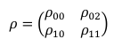
where ρ₀₀ + ρ₁₁ = 1 and ρ₀₁ = ρ₁₀. For a pure state, ρ₀₀ = |α|², ρ₁₁ = |β|², and ρ₀₁ = α ∗ β.

Bloch Sphere Representation

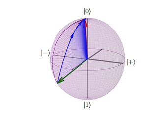
The state of a qubit can also be visualized on the Bloch sphere, where every point on the surface of a unit sphere represents a possible state of the qubit. The north and south poles of

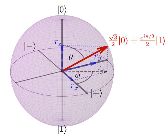
the sphere correspond to the states |0⟩ and |1⟩, respectively, while any other point on the sphere represents a superposition of these states. The Bloch sphere is a powerful tool for visualizing the state space of a qubit and the effect of quantum gates and quantum channels in general. 

Example of Bloch Sphere Representation, for the represented state θ = Φ = pi/3 .

There are multiple ways of defining the mapping of a quantum state to the Bloch sphere.

1. From Ψ: The quantum state |Ψ⟩ = α|0⟩ + β|1⟩ can be mapped onto the Bloch sphere by expressing the state vector's coefficients in terms of spherical coordinates:

where θ and Φ are the polar and azimuthal angles, respectively.

2. Using σ_x, σ_y and σ_z: These Pauli matrices play a crucial role in mapping quantum states onto the Bloch sphere. They are defined as follows:

The expectation values of these matrices with respect to the state ρ\rhoρ determine the coordinates on the Bloch sphere. The components of the Bloch vector r^→ = (r_x, r_y, r_z) are given by:

3. Link with ρ: The density matrix of a state whose Bloch vector is r^→ = (r_x,r_y,r_z) is:

One can see that a pure state is necessarily on the surface of the Bloch sphere, while a density matrix can also represent states inside the Bloch ball.

Entanglement

One of the most powerful features of qubits is their ability to become entangled with each other. Entanglement is a quantum phenomenon in which the states of two or more qubits become so interdependent that the state of each qubit cannot be described independently of the state of the others. This property is the basis for many quantum algorithms and protocols, including quantum teleportation and quantum cryptography.

The phenomenon of interest related to quantum entanglement in this context is the exponential expansion of the Hilbert space. Analogous to how classical bits exist in one of two states - either 0 or 1 - and a qubit may inhabit a complex superposition, representing a combination of both |0⟩ and |1⟩. For a system of N classical bits, the total number of possible configurations is 2^N, and a system of qubits can exist in a superposition encompassing all 2^Ν potential states simultaneously.

One can discriminate between separable and non-separable (or entangled) states. If a N-qubits state |Ψ_N⟩ can be represented as:

with |Ψ^k⟩ being a pure state of qubit k, it is said to be separable. Any state that cannot be put in this form is said to be non-separable.

For example,

is a separable state.
While 

is not.

A noteworthy example is the non-separable GHZ state: 

the GHZ state is sometimes referred to as the maximally entangled state.

Quantum Gates

Quantum gates are essential tools in quantum information processing, functioning as quantum analogues of classical logic gates. They perform operations on qubits and qudits, enabling the manipulation of quantum states, which is foundational for quantum computing and related technologies.

Types of Quantum Gates

• Single-Qubit Gates: These gates operate on individual qubits and include the Pauli gates (X, Y, Z), the Hadamard gate, and the phase shift gates (e.g., S and T gates). These gates typically act as rotations on the Bloch sphere, transforming the state of a single qubit.
• Multi-Qubit Gates: These gates operate across multiple qubits, creating entanglements and enabling more complex operations. The most notable among these is the Controlled NOT (CNOT) gate. Other examples include the SWAP gate, which exchanges the states of two qubits, and the Toffoli gate, an extension of the CNOT gate that operates on three qubits.

Implementing Quantum Gates

To implement a quantum gate, we apply the corresponding unitary matrix to the state vector or density matrix of the qubits. For example, if a quantum gate represented by the unitary operator U acts on a qubit initially in the state |Ψ⟩, the new state of the qubit is given by U|Ψ⟩. In terms of density matrices, the transformation is represented as UρU^†, where ρ is the density matrix of the qubit state.

A quantum gate U is the time-evolution operator of that qubit during a certain gate time t_g. If the gate starts acting on the qubit at time t₀, we have:

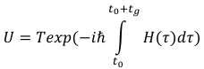
where H is the Hamiltonian acting on the system and T_exp is the time ordered time exponential.

Physical Realization

Implementing quantum gates in physical systems requires precise control over quantum interactions and the environment. Technologies such as superconducting qubits, trapped ions, and photonic systems are commonly used. Each technology offers different advantages and challenges, particularly in relation to gate fidelity, coherence times, and operational speeds.

A physical qubit realization is characterized by its Hamiltonian, which is generally composed of H_0 (the free evolution or drift Hamiltonian) and {H_k}k (an ensemble of control Hamiltonians). The total Hamiltonian that is plugged in is:

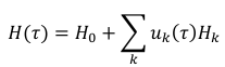
with uk(τ) being the control amplitudes of the Hamiltonian H_k.

To physically apply a certain gate on qubits, it is therefore a matter of finding the right control amplitudes given the physical constraints of the particular realization.

Quantum Algorithms

A quantum algorithm is a step-by-step procedure in which each step is implemented using a quantum gate. These algorithms are designed to operate within the quantum circuit model and exploit the unique properties of quantum states to perform computations.

Prominent Quantum Algorithms

• Shor's Algorithm: One of the most famous quantum algorithms, Shor's algorithm, factors large integers exponentially faster than the best-known classical algorithms. This capability has significant implications for cryptography.
• Grover's Algorithm: Grover's algorithm provides a quadratic speed-up for unstructured search problems compared to their classical counterparts. This algorithm is particularly useful for searching databases and solving optimization problems where no specific structure is exploitable by classical algorithms.

What is a Qudit?

A qudit generalizes the concept of a qubit to higher dimensions. While a qubit represents quantum information using two levels (typically denoted |0⟩ and |1⟩), a qudit extends this idea to d levels, where d can be any integer greater than 2. These levels are represented by the states |0⟩, |1⟩, |2⟩, . . . , |d − 1⟩.

State Representation

The state of a qudit is described in a d-dimensional Hilbert space. A general state of a qudit can be represented as:

where {αj}_j are complex coefficients satisfying the normalization condition 

Density Matrix Representation

The density matrix for a qudit is a d × d matrix defined as:

with the conditions that ρ is Hermitian (ρ^† = ρ), trace-one (Tr(ρ) = 1), and positive semi definite.

Generalized Bloch Representation

For qubits, the Bloch sphere provides a convenient visualization of the state space. In the case of qudits, the concept of the Bloch sphere generalizes to higher dimensions, often visualized through the use of generalized Gell-Mann matrices, which are the SU(ddd) analogues to the Pauli matrices of SU(2). Pure states of a qudit lie on a subset of the surface of a (d² − 1) dimensional sphere.

Quantum Gates for Qudits

Quantum gates for qudits extend the unitary operations applicable to qubits. A quantum gate that acts on a qudit is a d × d unitary matrix, allowing for a richer set of transformations due to the higher dimensionality.

Advantages of Qudits

The use of qudits in quantum computing offers several advantages. They provide a more compact representation of quantum information, as a single qudit can encode more information than a qubit. This compactness can lead to reductions in the number of quantum gates and the overall complexity of quantum circuits. Qudits can enhance the resilience of quantum information to certain types of errors and may offer advantages in quantum error correction.

Timescales

In quantum computing, the coherence of qubits - how long they maintain their quantum states - is fundamental for performing quantum operations. The timescales T₁,T₂, and T₂^∗ represent different aspects of how qubit states decay and dephase over time, directly influencing the performance and feasibility of quantum computations.

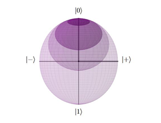
T₁: Longitudinal Relaxation T₁ time, often referred to as the longitudinal relaxation time, measures the time it takes for a qubit to return to its thermal equilibrium state along the Z-axis of the Bloch sphere. This process is also known as energy relaxation or spin-lattice relaxation, where an ensemble of qubits in an excited state |1⟩ relaxes to the ground state |0⟩ on its own in the interaction picture :

where E[⋅] is the average of the realizations. T₁. This time is critical for quantum systems, as it sets an upper limit on how long computations can run before the qubits lose their energy state.

T₂: Decoherence Time T₂, or the transverse relaxation time/decoherence time, describes how quickly the off-diagonal elements of a qubit's pure state density matrix decay. T₂ reflects the loss of quantum coherence due to the dephasing between the states of a qubit:

T₂ is generally shorter than T₁ and determines the time window within which the quantum gates can operate effectively before coherence is lost. 

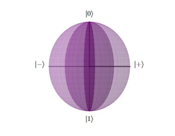
• Note: Figure 5 shows that pure dephasing can be interpreted as the transition to classicality, since at t -> infinite, the Bloch sphere becomes a simple line joining the two poles. Which means, the final state is indiscernible from an ensemble of classical bits that are either in |0⟩ or |1⟩.

There exists cases with T₂ > T₁, but T₂ ≤ 2T₁. A system where T₂ = 2T₁ is said to be "T₁ limited". And sometimes one can define 1/T_Φ = 1/T₂ − 1/2T₁ the pure dephasing time, that is, the supplementary dephasing time that is not due to the longitudinal relaxation.

T₂^∗ : Dephasing Time T₂^∗  represents the total dephasing time, including all sources of noise, not just those intrinsic to the qubit system. It is often shorter than T₂ due to additional dephasing effects from environmental instabilities. By changing the reference frame to the interaction picture and defining |±⟩:= 1/2 (|0⟩ ± |1⟩), and initializing the system in the state |+⟩ and letting it evolve, we define:

The difference between T₂ and T₂^∗ might not seem very obvious at first glance, and those two are often used interchangeably. It becomes even more confusing when one considers that, if ρ(0) = |+⟩⟨+|:

This makes it seem that T₂ = T₂^∗.

However, let us consider, that in the interaction picture of a unitary evolution, there is a non characterised interaction term H_I(t) = δ(t) |1⟩⟨1| -  it can be an external field noise, uncalibrated controls, etc. - that varies from one realisation to another, but can be represented by a Gaussian noise of variance 2/τ. Initialising the state in |+⟩ at time 0, and letting it evolve for a time t according to the Schrodinger equation, produces a system in the state 

This means that averaging over all the different realisations: 

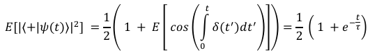
This is then a similar expression as before.

In reality, T₂ represents a type of decoherence that occurs because of non-unitary evolution. This means that it arises from interactions not described by the standard quantum mechanical framework of Hamiltonians within the system's Hilbert Space. On the other hand, T₂^∗ includes everything that T₂ covers, plus an additional dephasing term, similar to the Gaussian noise example we just saw. This extra term comes from averaging the effects across a group of systems. These systems undergo unitary evolution, meaning that they evolve in a predictable quantum manner, but they experience variations due to Gaussian noise or a normally distributed variation in their base Hamiltonian settings.

For instance, consider a qubit with two energy levels that are initially degenerate but are split due to a longitudinal field that has some noise in its control. Alternatively, imagine a group of qubits that are in slightly different environments. In such cases, the dephasing included in T₂* would account for these variations.

Finally, one could say that the total dephasing time T₂^∗ includes: the inhomgeneous dephasing time τ, the pure dephasing time Tφ (T₂ without the effect of T₁, see discussion in the T₂ subsection), and the longitudinal relaxation time T₁, as follows:

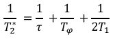
These timescales - T₁, T₂, and T₂^∗ - are essential for designing and evaluating quantum circuits, as they directly impact the error rates and practicality of implementing quantum algorithms. T₂^∗, as the limiting parameter, is crucial for any qubit system, especially particular type of qubit error, and each of those can be modelled by a specific quantum channel, in an open quantum system approach.